Chapter 8 Identifying pairs of features
The previous chapter explained that we can set our attention to process individual locations, or individual features. But we do poorly with combinations of features. The difficulty with encoding combinations of features, but not individual features, can be quite striking in some simple animations, as you will see below.

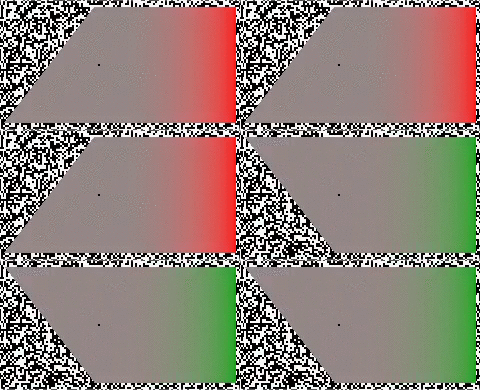
Figure 8.1: Try to perceive whether the red color is paired with leftward tilt or rightward tilt.
If the animation above doesn’t work, watch it here.
What’s going on in the above animation should be easy to perceive - the color is alternating between green and red, and the left side edge is alternating between leftward-tilted and rightward-tilted. You can also easily see how the features are paired; that is, when the left side is leftward-tilted, the right side is red.
Speeding up the alternation of the two frames can reveal the time it takes for our brain to combine features (A. O. Holcombe and Cavanagh 2001).

Figure 8.2: Try to perceive whether the red color is paired with leftward tilt or rightward title.
If the movie above isn’t viewable, watch it here. At this fast rate, note that it is still easy to see that the individual features are red/green and left/right, but it’s hard to judge which occur at the same time. The brain takes too long to identify combinations of features to know which were presented simultaneously.
The previous chapter explained that we can select objects in the scene by certain individual features such as by location and by color. For example, we can think “red” and our attention will process all the locations containing red more. However, this doesn’t work for combinations of features such as red and leftward-tilted. The present chapter showed another side of our trouble with combinations of features - simply identifying pairs of features can be quite time-consuming.
To experience that more, watch the below two-frame animation. This time, the challenge is to combine two different orientations. At the slow rate (top row), you can do it. But in the middle row, you may not have enough time. If the animation doesn’t show, try watching it here.

Figure 8.3: For each row, try to perceive whether the leftward tilt on the left is presented at the same time as the leftward tilt on the right.
Feature pairing can also be time-consuming for color with motion direction, as illustrated by the animation below.

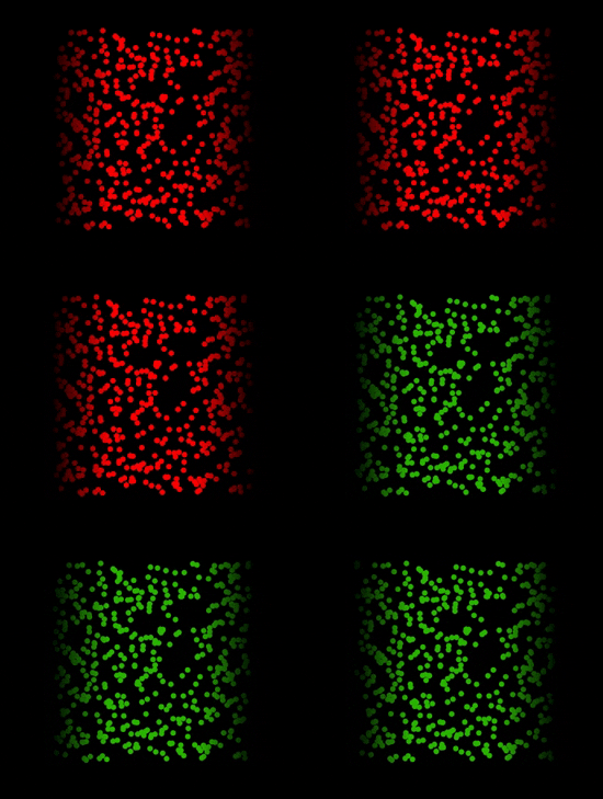
Figure 8.4: For each row, try to perceive whether the dots, when white, are moving to the left or to the right.
While at the slow rate of the top row, it is easy to judge the pairing of motion direction and white/black color, it’s difficult in the middle row, where the speed is slightly faster (Alex O. Holcombe 2009).

Figure 8.5: At this rate, most who aren’t color blind can easily perceive the direction of motion when the dots are green.

Figure 8.6: At this faster rate, it’s difficult.

Figure 8.7: At this very fast rate, none of the people tested in the lab could do it. If you blink, though, you can cheat.
In the previous chapter (7), you learned that our brain has a process for attentional selection of an individual feature value (such as blue), but not for combinations of features. Consistent with this, the animations of this chapter illustrate that identification of feature combinations is time-consuming. This suggests that identifying features requires capacity-limited (post-bottleneck) processing. In the next chapter, we will put these ideas together to better understand classic findings from visual search experiments that you learned about in first-year psychology.
8.1 Exercises
Answer these questions:
- What does the slow limit on pairing simultaneous features have in common with what was said in the previous chapter about selection?
- How do the demonstrations above relate to Learning Outcome #6 (2)?